
Size and Age in the NHL, Pt. 5
Size and Age in the NHL, Pt. 5
Predicting Playoff Success from Biographical Matchups

Following up on my examination of the relationships between size and age and playoff success, I thought it would be a fun, interesting exercise to try a variety of predictive models based solely on the size and ages of the teams matching up. This is essentially the same idea as the models I tested at the end of my look at the regular season. I try to model which team wins a game based solely on the difference in age and size between the teams. To make things easier, I focus on all situations instead of breaking things down by strength state and look at each game from the home team’s perspective. I use the same positional differences that I used for Part 4, that is Age, Height, Weight, and BMI for Forwards, Defense, and Both, resulting in up to 36 predictors.
In contrast to my analysis of regular season point totals, where I used the entire dataset to train and evaluate my models, this time I partitioned my data into an 80/20 split between a training set and a test set.
Logistic Regressions
The first model I tried was just throwing all the predictors together in to see what came out. Somewhat unexpectedly, this resulted in sixteen variables being removed from the regression due to singularities: all the the defense-to-defense, defense-to-both, both-to-defense, and both-to-both differentials. This was confusing. I knew from doing my correlation analysis that none of the predictors were perfectly correlated with each other. After some Googling, though I realized that predictors that can be inferred from some combination of other predictors would be removed, which was what was happening here.1 This makes sense in retrospect, but it had not crossed my mind when I was putting the model together. A bit of messy start, but nevertheless, I forged on.

Of the indicators that remain, an interesting pattern emerged; the coefficients seems to balance each other out. In this case, the F-F and D-F differences group on one side of zero with the F-Both difference, while the F-D and Both-F differences are on the other side and Both-F is quite far in the other direction. I actually ran all the code for this post twice with different train/test sets by accident because my workspace crashed and I didn’t initially make sure that my train/test partition would be repeatable and the same pattern occurred then too. Well, I thought, perhaps this is an effect of throwing everything into the model at once. Perhaps when I try to isolate differences by limiting which home team position the opposing team is compared I’ll find a meaningful pattern.
However, breaking the models down by position of the home team does not reveal much of a difference from throwing everything in at once.

Roughly the same pattern occurs as the previous model: two of the home to away position comparisons for each metric are on one side of zero and the third is on the other side of zero and roughly equal to the sum of the first two. Even more curious, for almost every biographical metric, the same positional comparisons group on the same side of zero, with the exception of weight and the home defense model.
Two things to pay attention to before moving on to the next section. First, when I reduced the number of predictors, the magnitude of the coefficients was reduced as well. I believe this is an indication of a very noisy mess of indicators basically cancelling each other out and ratios of the predictors to each other getting more precise (though maybe not more accurate). I think this is supported by the two on one side of zero, one twice as far on the other side of zero pattern that’s shown up consistently so far. Second, age has had basically no effect with the coefficients for age hugging the zero line on the charts so far.
Penalized Regressions
Previously I performed manual feature selection; basically a combination of what I thought made sense and which features were least correlated with each other. However, penalized or regularized regression can perform this process automatically. I tested three methods of penalized regression: ridge regression, lasso regression, and elastic net. They are all variations of the same process, the difference between them is essentially how aggressively they zero out coefficients in the final model. Ridge regression is the least aggressive in setting coefficients to zero and doesn’t zero any out. Lasso regression is the most aggressive zeroing out coefficients. And elastic net is a method that balances the two based on a variable alpha that can range from zero (lasso) to one (ridge). To find the alpha value for the elastic net regression, I used the train() function in the caret package to test values incrementing by 0.1 and selected the model that performed best on the training set. In this case, a value of 0.3 performed the best. For ease of interpretation, I removed any coefficients that had been set to zero.

The first thing that really stands out is that the lasso regression really was aggressive in shrinking and zeroing out coefficients. Only three were not set to zero, and they are all very close to zero. This is probably yet another indication that there is not much predictive value in the biographical makeup of teams in the playoffs. Age is once again at or near zero for all the models tested. Once again the pattern of the predictors nearly balancing out for each biographical metric emerges again as well.
XGBoost
Finally, just for fun I decided to try to train an XGBoost model as well. I’ve never used XGBoost before, so I thought this would be a good, relatively simple problem to learn on. XGBoost is the algorithm behind several popular hockey models including Evolving Hockey’s xG model and MoneyPuck and Patrick Bacon’s models, I believe, as well as game prediction models. XGBoost is also pretty well known for performing well at Kaggle competitions and is considered one of the top current classification models. Since a binary outcome is the simplest possible classification problem, it lends itself to this project well, in theory.
A super high level description of XGBoost is that it is an extension of decision tree and random forest models that utilizes gradient boosting to determine how to weight the different trees in its forest. There are a lot of tuning parameters for XGBoost and since I didn’t have much practical familiarity with them prior to attempting this, I did what I did with the elastic net model and used a tuning grid/matrix to select the model that performed best on my training set.
XGBoost does not output coefficients the way logistic regressions do, however it does include information gain for each predictor. I included the top twenty, although it reaches zero information gained well before reaching twenty variables.

In a notable departure from previous models, age seems to be the second largest source of information gain behind height! Very interesting! It’s nice to see some disagreement. Let’s see if XGBoost knows something the other models do not.
Model Comparisons
To compare the models, I ran each of them on my test set and calculated the log loss, R-Squared value, and root mean squared error for each model.
In addition to the models already described, I included a model that I call Logistic (Intercept Only), which was a logistic model with no predictor variables. In practice, this means it just uses the home team’s win percentage in the train set as its prediction for everything in the test set. I used this as the baseline for evaluating all the other models.
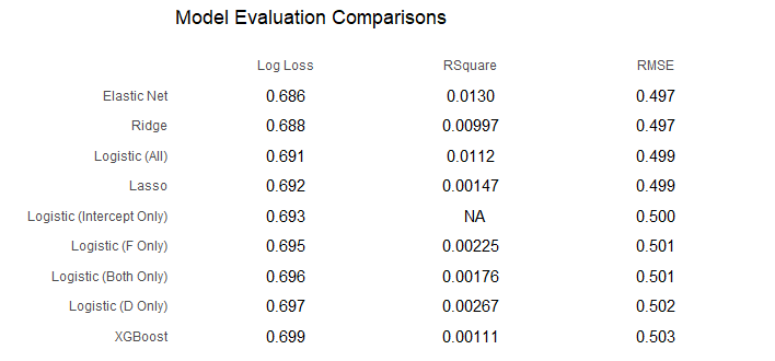
It turns out XGBoost did not uncover something the other models were missing. Instead, it performed the worst of all, possibly the result of overfitting since I may have been to granular in testing values in the tuning grid. All three penalized regressions outperformed the baseline, although just barely for the lasso model. That’s not surprising though, since the lasso model was barely more than than just the intercept. Elastic Net performed the best, although the difference between it an the XGBoost model were really small. Looking at the R-Squared values, none of the models explained more than about 1.5% of the variance in outcomes and most did significantly less than that.
Somewhat surprisingly, the positionally specific logistic regressions all did worse than the baseline while the everything-and-the-kitchen-sink logistic model did better. The differences are so small that it may not mean much, but this was a consistent result between both my runs through the code.
Conclusions
It’s probably not a surprise seeing as this is part 5 of this series, but it seems safe to say that age and size don’t matter in the playoffs. Not at the team level, at any rate. Neither age, nor height, nor weight, nor BMI will help you predict the winner of a playoff game any more accurately than just knowing who the home team is. For the next part of this series, I plan to look at size and age and how that correlates to player performance at the individual level. However, depending on my own time and availability, I might choose another topic I think I can knock out more quickly.
Fin.
A huge thank you goes to Evolving-Hockey for providing team, player, and even play-by-play data in a clean, easy-to-use format. When I did my last major project I was combing through the NHL play-by-play data up till 2017-18 and it was quite messy. Fortunately, Evolving-Hockey absolutely has the best quality of any of the major hockey stats sites I’ve looked at and it makes hobbyist work like this so much easier. For that reason, although I’ll use their data and make some of my data available, I won’t include anything from their site that can’t also be found on NHL.com or other free sites.
For example, if I have a-c, a-d, and b-c, I can find b-d, with (b-c) + (a-d) - (a-c)
Great Work!
Great work!